Estimation of Wind Energy Production

Overview

The calculation of the wind resources on-site and the corresponding energy production are based on the assessment of wind potentials by anemometric measurement. The wind data is processed by software packages to calculate the expected wind energy yield for the proposed site.

Meteorology

Generally, wind flows are large-scale balancing air movements in the atmosphere between high pressure and low pressure-areas, in some cases superposed by local balancing movements. The pressure differences are caused, and driven by, the solar heating of the Earths atmosphere, landmasses and water bodies. Warm air is rising, leaving a low pressure area at the surface and causing high pressure areas within higher layers of the atmosphere where the air is cooling down and falling to lower layers with respective pressure effects.

Since the balancing air movements also run near the earth's surface they are significantly affected by the surface roughness and the orographic terrain structure.

Roughness is a quantitative description for the friction of the surface causing a slowdown of the near-surface air flow. Water and land without vegetation has a low roughness and therefore a minimal effect to the wind, forests or cities have a high roughness.

On top of a hill, the air flow is compressed and thus the wind has a higher energy density compared to the same air flow over flat terrain. Furthermore, valleys and similar terrain structures can act as a blast pipe, concentrating the air flow. Behind mountain ridges and inside valleys the air flow is disturbed by recirculation and shading effects.

Software Basics

WindPro

The WindPRO philosophy is object orientated projecting. A wind park project consists of a number of objects, whereby the wind turbines are key elements. Objects are: wind turbines, wind monitoring stations, local obstacles etc. Some of the objects directly determine the wind energy, others focus on the environmental aspects and yet some others can also influence the feasibility of the project. The characteristics of the objects are combined with the terrain data such as the surface roughness maps and the height level contour lines and serve as basic input data for the energy calculations with WAsP, which is the WindPRO integrated meteorological simulation model.

WAsP

WAsP is a software program for predicting wind climate and energy yield of wind turbines. The predictions are based on wind data measured on site or from stations in the same region and considers the effects of the surrounding terrain to the wind flow (topography, surface description, obstacles). WAsP uses the wind atlas methodology. In a first step the influence of the terrain to the wind flow is calculated, creating a generalised regional wind climate.

In a reverse process, this generalised regional wind climate (called wind statistic) is then applied to topography, surface description and obstacles at the vicinity of each individual wind turbine, providing the wind flow at this point even if the wind data has measured in some distance which can be, depending on the terrain, up to several kilometres.

Model Input Parameters

Besides the processed wind data, important input parameters for the energy yield calculation model are as described the terrain description, comprising of the orographical (topographical) model and the description of the earth´s surface (roughness description).

Orography

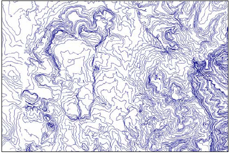
A method to gather data describing the orographical terrain is the analysis of data collected by satellites. As an example the SRTM -Shuttle Radar Topography Mission data base – provided by the US Geological Survey – scanned the earth´s surface between 60° latitude north and 54° latitude south, with a resolution of 90 x 90 m.

The data in between these points can be interpolated using the WindPro software to gain the topographical model of the proposed site, with a height contour density of 5 metres, as shown in Figure 1 (the example shows the orographic map of the Ashegoda site in Ethipia, where a feasibility study for a wind park has been conducted by German Technical Cooperation (GTZ)).

Figure 1: SRTM height contour map of Ashegoda wind park site in Ethiopia

Besides this advanced method of gathering topographical data, national or regional institutions can be asked for topographical maps of the area. The developers have to take care, whether the maps are available in an appropriate scale. Sources should be compared regarding accuracy and potential failures.

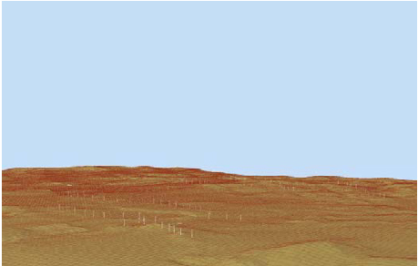
The height data is than processed to a three-dimensional digital elevation model of the wind farm site. An example for the Ashegoda site is shown in figure 2.

Figure 2: Three-dimensional digital elevation model of Ashegoda site, view from south-western direction

Roughness

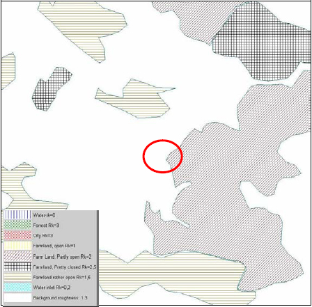
For the model simulations the roughness classification for the surface in close proximity to the wind farm site is derived from topographical maps, data obtained during site visits as well as aerial photos of the region. A basic description of the roughness classes is given in the following (roughness length is a second roughness description unit), it has to be noted that the roughness class is a defined value which can not be measured directly. The roughness length describes the height where the wind speed in a logarithmic wind profile is becoming zero; the coarser the surface, the higher the roughness length.

Roughness class	Roughness length	Relative energy	Description of surface
0	0,0002	100	Water areas
0,5	0,0024	73	Mixed Water and land area of very smooth land
1	0,03	52	Open farmland with no crossing hedges and with scattered buildings. Only smooth hills
1,5	0,055	45	Farmland with some buildings and crossing hedges of 8m height and about 1250 m apart.
2	0,10	39	Farmland with some buildings and crossing hedges of 8m height and about 800 m apart.
2,5	0,20	31	Farmland with some buildings and crossing hedges of 8m height and about 250 m apart.
3	0,40	24	Villages, small towns, very closed farmladn with many or high hedges, Forrest, many abrupt orographic changes.
3,5	0,80	18	Large towns, cities with extended build-up areas
4	1,6	13	Large cities with build-up areas and high buildings

As an example for a roughness description the map of Ashegoda site is presented in the following Figure 3.

Figure 3: Roughness map for Ashegoda wind park site in Ethiopia

Wind Shear

In many assessments of the wind potential the upper anemometers of the wind measurement are installed at a height of 40 m above ground while the hub height of modern wind turbines today often reaches heights between 55 m and 60 m above ground level. To estimate the wind regime at hub height of the wind turbines (the WAsP model simplifies the wind speed distribution over the rotor as concentrated to the hub height) the wind speed is extrapolated according to the following formula:

Whereas γ is the Power Law Exponent or Wind Gradient which is depending on the roughness of the terrain, the thermical lamination of the atmosphere, the wind speed itself and the height above ground. The exponent must be calculated sectorwise for the wind park site. This can be done by the WindPro-Software package from the measured wind data at the heights of 10 m a.g.l. respectively 40 m a.g.l..

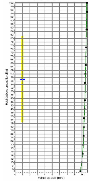
The wind gradients for the twelve wind distribution sectors describe the wind speed at different heights for all wind directions diveded in sectors of 30°. An example for a calculated wind profile (increase of the wind speed with height) for the main wind direction of this site (sector south-southeast) is displayed in Figure 4.

Figure 4:Wind profile of Ashegoda wind park site (main wind direction south-southeast)

Combining considerations of terrain and roughness, the wind profile for the area of each individual wind turbine is then calculated by WAsP. The extrapolation from 40 m measuring height to 60 m hub height can be considered as reasonable but a further increase of the wind speed for hub heights of 80 m and more is not stringent as the power law is not suitable for height extrapolations over this range.

Wind Turbine Parameters

To estimate the performance of different turbine types for the development of a new project usually several scenarios using different turbine types are calculated. Important turbine parameters, which should be included are hub height, nominal power and rotor diameter.

Power Curve and Air Density

The Power curve of a wind turbine is an important parameter, describing the relation between the wind speed on site and the respective electrical energy output. Power curves and ct-values (a parameter for the calculation of the wake effect) of the turbines under consideration are applied for the energy calculation. Power curves which had been measured by independent institutions are of higher quality than calculated ones. Due to the fluctuations of both the characteristics of the wind turbine components, and the measuring conditions power curves of different measurements differing slightly between each other.

Several manufacturers are thus providing power curves which are calculated from the results of several measured ones; the performance of these calculated power curves might be contractually guaranteed by the manufacturers.

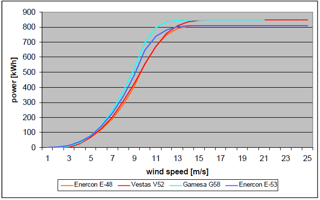
During the calculation of the energy yield, the power curves, given for the standard conditions of air density = 1.225 kg/m³ are adapted to the air density of each individual turbine location at hub height, with the transformed power curves for the average air density. The air density can be calculated by WindPro for each individual wind turbine according to the site conditions, height above sea level plus the hub height of the turbines (e.g. 57 m / 60 m) and an annual average temperature level. As verification, the calculated adaptations for air density at the turbine sites should be compared to information provided by nearby meteorological stations. Figure 5 shows the power curves of several wind turbines at an air density of ρ = 1,225kg/ m³.

Figure 5: Power curves for wind turbines proposed for the Ashegoda wind park in Ethiopia

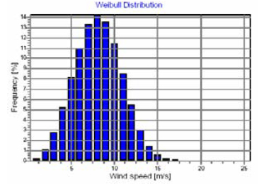
As can be clearly seen, the Enercon E-53 and Gamesa G-58 wind turbines are generating more energy in the wind speed range from about 6 m/s to 12 m/s which occur more frequently then the other wind speed ranges, see the Weibull-distribution in Figure 6 This is mainly caused by be larger rotor diameter compared to the Enercon E-48 and Vestas V52 wind turbines.

Figure 6: Weibull distribution for Ashegoda wind project site

Losses and Uncertainties

Meteorological phenomena can only be predicted to a certain limited degree. As a consequence it is not possible to make an exact forecast of the wind conditions even if longterm reference data (which can only represent the past) is used. Furthermore, data collection and processing is always afflicted with errors and inaccuracies as is every mathematical or physical model used to describe or predict real procedures. To compensate the inaccuracies in modelling approach and basic input data, it is advisable to use factors of safety to adjust, or discount the final output. Two blocks determine the factors of safety: losses and uncertainties.

Losses

Losses are found on the whole energetic transformation chain from the rotor (kinetic energy) to the substation (electrical energy). The losses are simple add-ups to the total reduction of the calculated energy yield. In detail:

Park Efficiency

After passing the rotor of a wind turbine, the wind has a decreased speed due to the kinetic energy taken away by the rotor and increased turbulence caused by the rotating rotor and the difference in speed compared to the undisturbed flow. Until the speed difference to undisturbed flow is not equalised, the result is a lower energy yield for the wind turbines following in the direction of the flow. These losses are called array or wake losses.

Turbine Availability

The turbine availability is the percentage of a year (i.e. 8760 hours) where the turbine is able to generate electrical energy while being connected to the grid. Reasons for the non-availability of a wind turbine are various, and include downtimes for regular maintenance and servicing, component failures (including defect sensors), overheating of components, repairs or exchange of components, as well as errors and downtimes of the superior electrical grid. The turbine availability can be set to a value by taking into account the experience in the operation of windturbines in the region and skills of local staff. For a country without experiences and a high need for capacity building during the first years of a project a standard value of 95 % can be applied. Later on and after the first years of sufficient turbine availability averages, the aim should be to raise the level up to 97 % which could be seen as a good value for the first wind parks in a country with few experiences in wind turbine operation. A common value for countries with a very established wind energy industry, an availability of 98 % is assumed.

Electrical Losses

The electrical losses depend on the resistance of the conductors and on the current intensity. To assess the current intensity of the wind park the following methodology is used: the duration curve of the wind park for one year is approximated by a two stage approach. For 10% of the year (876 hours) full power is assumed and for the rest of the year (7,884 hours) the load is estimated to 25% of full load.

For this power pattern of the wind park, the turbine current is derived and the losses for the internal wind park cabling, and for the wind park cabling connection to the substation are calculated relative to the total energy output.

For the Ashegoda wind park in Ethiopia the following values have been calculated:

• internal park cabling: 0.2%
• internal park transmission lines: 0.5%
• turbine transformers: 1.1%
• transmission line 230kV: 0.5%
• substation transformer 0.5%

The total electrical losses of the park are estimated at 2.8% of that amount of electricity which is produced by the wind turbines.

Miscellaneous Losses

In addition to the transmission losses and lost production due to reduced availability a number of other losses should be taken into account. The aerodynamic turbine performance described by the power curve is strongly depending on the profile and surface of the wind rotor blades. Blade fouling from dirt or insects on the surface of the blades lead to non-expected change of airfoil characteristics and to lower energy yield. Whether a change of blade characteristics has to be expected, depends on climatic conditions like humidity. For example an average air density of a temperature of 17° in 2.400 m above sea level provides no thermal problems for the wind turbines. No effect of the low air density is to be expected than the reduced energy production.

High wind control losses are caused by the turbine cut-in and cut-out strategy. The turbines will cut-off when cut-out wind speed is reached and will not re-cut-in until wind speed is below a defined wind speed level, lower than the cut-out level. A reduction factor of 0.1% to the gross energy output was applied to take these effects into account.

Wind Speed related Uncertainties

Uncertainties cover the inaccuracy of the data processing from the measurement, the internal data processing and the long-term prediction. A percentage value describes the standard deviation of scattering results around the expected true value. For the energy calculation, these wind speed-related uncertainty values have to be transformed to the energy production level. Additional uncertainties have to be determined for modelling and mathematical algorithms.

Uncertainties of the WAsP-Model

The WAsP (Wind Atlas Analysis and Application Program) software is a proven tool used in the wind industry for more than 15 years. As every model it has limitations and uncertainties mainly due to the simplifications behind it which had been done to handle the calculations on desktop computers in an acceptable time frame. Mesoscalic meteorological models require powerful computers and a calculation time of several days. However, WAsP has been used for a considerable time worldwide and the uncertainties have been evaluated over the years. In case of Ashegoda, the existence of modestly shaped hills and ridges lead to a suffiecient quality of the calculation.

• Transfer Wind to Energy
  The discrete wind flow from discrete wind directions is simplified to 10-minute average values for 12 direction sectors and statistically preprocessed before being applied to the power curve.
• Site modelling
  Consists basically of two input parameters: the topographical model and the surface description (roughness description).
• Flow modelling
  WasP has been developed for use in areas with only modestly shaped hills which is the case at Ashogoda site. The uncertainty of the flow modelling is set to the medium value of 3.0% .
• Wake modelling
  The uncertainty of the selected wake model will be low, if the area of the wind farm itself is nearly plain (no additional uncertainties due to the influence of the terrain). In case a high roughness length is found for the terrain, the uncerainty in wake modelling can be much higher.

To calculate the total uncertainty all single uncertainties can be considered as stochastically independent and the commonly used way of estimating the joint uncertainty of independent (un-correlated) uncertainties is to calculate the RMS (root mean square) value.

Uncertainties of the Wind Data

The reliability of the WAsP calculation is highly dependent on the quality of the input parameters of which wind data is the most important one. The collection and processing of wind date is subject to several uncertainties.

• Anemometer calibration
  Anemometers should be calibrated in order to secure that the measured wind speed equals the actual wind speed.
• Anemometer characteristics
  Describes the uncertainty of the quality the anemometer detects the wind flow and processes the values to digital data.
• Mounting error
  The anemometer has to be vertically mounted. The uncertainty describes the effect if this is not done properly.
• Data recording
  Describes the uncertainties related to processing and storage of the data provided by the anemometer and the wind vane in the data logger.
• Terrain description
  Describes the uncertainty of the influence of the terrain to the measurement. Inclined wind flow and strong turbulence can not be measured accurately by a cup anemometer.
• Long term correlation
  The data used for the long term correlation as well as the MCP-Process includes uncertainties;

To calculate the total uncertainty all single uncertainties can be considered as stochastically independent and the commonly used way of estimating the joint uncertainty of independent (un-correlated) uncertainties is to calculate the RMS value.

Uncertainties of the Power Curve

It has to be considered that the power curve used for the gross energy calculation is also subject to uncertainties which had been described in the section 'Power curve and air density'. Due to the non linear relation of mean wind speed and energy these uncertainties can not be integrated into the uncertainties of wind conditions but have to be dealt with separately. In the following section an example for the calculation of the uncertainties of the energy yield for one wind turbine type is given.

The uncertainty of the power curve is, assuming the power performance of the turbine as independent of the energy deviation due to wind uncertainties, connected to the uncertainties of the energy yield by the following equation:

The turbine supplier usually gives a guarantee of 95 % of the energy values, which leads to an uncertainty to the predicted figures of 5 %; the actual guarantee value has to be negotiated with the manufacturer, the uncertainty can be adapted accordingly. This figure has been taken for every wind turbine type as it is sufficiently conservative for both calculated and measured power curves.

Uncertainties Energy Yield

The interpretation of uncertainty in energy yield from the total uncertainty in wind speed is not straightforward. The theoretical cubic relation of wind speed and energy does not give a correct description of the phenomena.

For the long term mean wind speed averaged over all turbine locations at hub height the average wind speed value is derived from the wind data processing. The uncertainty is equivalent to a reduction to the mean wind speed when considering the worst case. To translate this reduced mean wind speed into energy yield the parameters of a Weibull distribution are adapted and this new Weibull distribution is then applied to the individual turbine power curves. The results for the considered wind park layout can be found in the examinations in the following tables Deviation of Energy due to wind uncertainties, indicating an energy deviation due to the uncertainty in wind speed assessment.

Calculation of uncertainties in energy yield for a specific wind turbine

The transformation of the wind speed related uncertainties into the energy related uncertainty by appropriately reducing the wind speed at hub height leads to the following results:

	Mean wind speed [m/s]	Deviation wind speed	A-factor [m/s]	k-factor	Energy Yield [MWh/y]	Deviation Energy
calculated WAsP	8,84	0,0%	9,81	3,62	248,854	0,0%
reduced wind speed; uncertainties taken into account	8,35	5,6%	9,26	3,62	218,642	12,14%

Assuming the power performance of the turbine as independent of the energy deviation due to wind uncertainties, the total uncertainty for energy yield can be determined from the uncertainties of wind conditions and power curve.

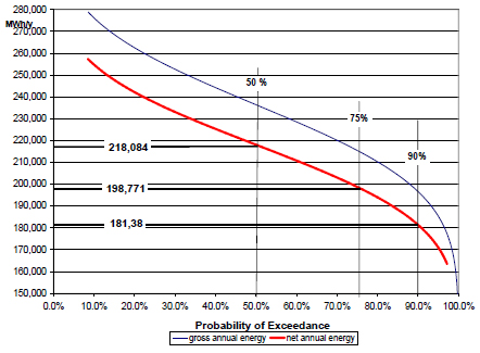
The analysis of uncertainties is an important step for the risk assessment of the project. From the predicted annual energy and from the total uncertainty on the energy level the probability of exceeding of certain energy yields can be calculated by statistical methods. Applying a Gauss process for the statistic analysis, the calculated gross annual energy can be understood as the mean annual energy yield having the highest rate of probability of all single results. The uncertainty shall be understood as standard deviation of the expected results around the most probable event.

Figure 7 displays the probabilities that a certain amount of annual electricity production is exceeded for the example wind turbine.

Figure 7: Probability of exceedance of certain energy yields for Ashegoda wind park

Gross annual energy describes the energy yield as calculated and net annual energy the energy yield considering the losses and uncertainties.

Besides the uncertainties for wind conditions and power curve, the losses for electricity transmission (e.g. 2,8 %) and reduced availability of the turbines (e.g. 95 %) have also to be considered as constant factors, reducing the estimated energy yield.

Further Information

• Wind Portal on energypedia
• Assessing Wind Potentials

References

- ↑ The contents of this article have been prepared by the project team of the feasibility study of the Ethiopian wind park Ashegoda, conducted by the Deutsche Gesellschaft für internationale Zusammenarbeit (GIZ) in cooperation with the Austrian development agency and Lahmeyer international. Originally the contents have been published as: GTZ (2006) Feasibility Study for Wind Park Development in Ethiopia and Capacity Building - Ashegoda Wind Park Site), retrieved 11.7.2011 [[1]]
- ↑ EMDinternational (2010) WindPro users manual, retrieved 26.7.2011 [[2]]
- ↑ Mortensen N. G., Landberg L., Troen I.,fckLRPetersen E. L., Rathmann O. and Nielsen M.(2004) WAsP Utility Programs, retrieved 25.7.2011 [[3]]